Chain mapping
Excerpt: Students are led to an understanding of what the chain rule means and why it works, using mapping diagrams. It builds on two earlier mapping diagrams resources.
Warm-up
In Mapping a function, we explored mapping diagrams for linear functions. What happens if we now compose two functions?
-
How could we draw a mapping diagram to show the composition of the function with the function to get the function ?
-
We described linear functions as scalings. How are the scalings represented by the three functions , and related to each other?
Warm-up ideas
In Mapping a function, we explored mapping diagrams for linear functions. What happens if we now compose two functions?
- How could we draw a mapping diagram to show the composition of the function with the function to get the function ?
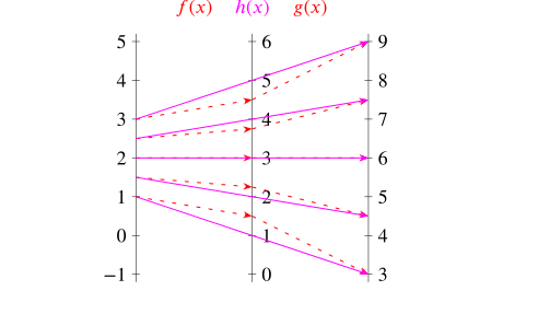
We can represent this composite by using three numberlines, with arrows from the left to middle one representing , and then arrows from the middle to the right representing , like this:
Here, we have centred the left-hand numberline on ; the numberlines are centred in such a way that the arrow starting from is horizontal, as before.
We can then show the composite function by joining the starts to the ends of the arrow chains, like this:
This shows how the function takes values from the left-hand numberline to values on the right-hand numberline.
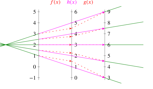
As in Mapping a function, we can also extend the arrows beyond the numberlines. For clarity, we only do this for the composite function :
The lines all meet in a point, showing that is a scaling with a scale factor of . (This is the scaling factor from the left-hand to right-hand numberline.) As , this is to be expected.
We can also check that the formula we worked out in Mapping a function for the location of the focal point gives us the expected location: that formula gives the location as times the distance between the numberlines. This matches what we see in the diagram, because the numberlines of interest here are the left-hand and right-hand ones.
- We described linear functions as scalings. How are the scalings represented by the three functions , and related to each other?
is a scaling with scale factor and is a scaling with scale factor . The composite function is a scaling with scale factor .
In general, if we compose a scaling with scale factor together with a scaling with scale factor , we will get a scaling with scale factor . In our particular case, we have .
Here, we used linear functions with no constant term and centred our mapping diagram on . Would we have obtained the same results if we had started with the functions and , still with , and centred our mapping diagram on (as input value)?

Problem
In Mapping a derivative, we saw that we can think of a derivative as a local scaling. What happens if we now want to find the derivative of a composite of two functions?
-
What does the mapping diagram of the composite look like if and (so that ), and we centre our mapping diagram at on the input numberline?
-
How does the diagram change as we zoom in?
-
What does this tell us about the derivative ?
-
Generalising this, given any composite function , how can we find for a given ?
You can download blank composite mapping diagrams with one on a page or two on a page, or you can use the interactivity to explore this.
Things you might have noticed
If we draw the mapping diagram at a scale of unit per tick mark, we obtain the following, where the non-linear behaviour of is clear, though that of is less so:
We can now draw the composite arrows and extend them into lines:
We see that the green lines fail to meet at a point. If we zoom in, things now look very different:
What is going on here?
-
The composite function appears to be a local scaling, as all of the lines meet at a point. From the diagram, the scale factor appears to be .
-
The function is locally a scaling with scale factor . We can see this either by looking at the mapping diagram carefully, or by noting that the derivative of is , so that the scale factor at is .
-
The function is also locally a scaling when we zoom in. The scale factor is a little harder to make out reliably from the diagram, but we can use what we know about differentiation to calculate it. We have . The function is centred on in this diagram, so the local scale factor is .
-
Composing these, we obtain a local scaling with scale factor , multiplying the scale factors as we saw in the Warm-up section. This calculated composite scale factor agrees with what we observed about the function .
So we conclude that .
Here is a somewhat generic sketch of a composite mapping diagram for , where we have shown the arrows and lines for but not for the individual functions or :
The function gives a local scaling with scale factor , the derivative of at .
The function is centred on , so it gives rise to a local scaling with scale factor , the derivative of at .
Since is locally the composition of these two scalings, we see that is also a local scaling. The scale factor of the composition is the product of the scale factors of and , so .
This is the chain rule, which can therefore be written:
There is another common way of writing the chain rule, which we can get by setting and , so that . We then have and , which we can write as . Substituting this into the previous version then gives us:


Interactivity
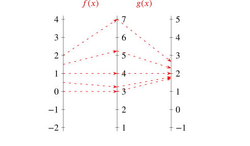
To enter the function into this applet, type x^2. To enter , type sqrt(x).
[interactive embed (geogebra-iframe): //www.geogebratube.org/material/iframe/id/R8RFvC2q/width/600/height/493/border/888888/rc/false/ai/false/sdz/false/smb/false/stb/false/stbh/false/ld/false/sri/true/asb/false/at/html5] — not part of the text import; see the source page.
Download GeoGebra file