Core Practical: Investigating Specific Heat Capacity
4 guided lessons · 36 checks · 5. Solids, Liquids and Gases → Changes of State
Guided lessons for this note
Which concept don't you understand yet?
We'll explain it simply and check your understanding. Pick any lesson — any order works.
0 of 36 checks correct so far
Lesson 1 of 4
Aim and variables of the SHC investigation
The aim is to measure a specific heat capacity from first principles: supply counted electrical energy to a known mass and watch the temperature respond. Naming the variables precisely is what turns a heating demonstration into a fair test.
What you know already
Here the ΔQ = mcΔT equation is turned around and measured, not just used. An immersion heater delivers counted joules into a known mass, a thermometer logs the rise, and the gradient machinery of the plotted graph yields the capacity of water or a solid block — with honest error analysis attached.
Key points of understanding
- The aim is to determine the specific heat capacity of water or a solid material.
- The independent variable is the energy supplied by the heater.
- The dependent variable is the temperature rise of the material.
- The mass of material and the starting temperature are controlled variables.
- Energy supplied is computed from the heater's voltage, current and heating time.
Choose a confidence level to continue.
Prefer to read it all at once? Show the full lesson as a page
1.Aim and variables of the SHC investigation
The aim is to measure a specific heat capacity from first principles: supply counted electrical energy to a known mass and watch the temperature respond. Naming the variables precisely is what turns a heating demonstration into a fair test.
Key points
- The aim is to determine the specific heat capacity of water or a solid material.
- The independent variable is the energy supplied by the heater.
- The dependent variable is the temperature rise of the material.
- The mass of material and the starting temperature are controlled variables.
- Energy supplied is computed from the heater's voltage, current and heating time.
First pass
Heat a known mass with an electric heater, count the energy from voltage times current times time, and measure how many degrees the mass climbs. Divide the energy by the mass and the rise to get the capacity.
Analogy — Metering a taxi journey: the meter (heater) counts the fare (energy), the passengers (mass) and distance (degrees) are known, so the per-passenger-per-kilometre rate (capacity) can be worked out.
Exam pointer — Variable-naming marks are free if you keep the roles straight: energy supplied is what you change, temperature rise is what you measure, mass is what you hold fixed.
Going deeper
The design computes ΔQ as VIt from ammeter and voltmeter readings timed with a stopwatch, so the energy is known without calorimetry assumptions. Controlling the mass pins the proportionality between energy and temperature rise, and the starting temperature is held near room value to limit unquantified exchange with the surroundings.
Analogy — Calibrating a fuel gauge by driving a known distance at a metered flow: fix the tank size (mass), count the litres (energy), read the needle (temperature), and the car's thirst per kilometre emerges.
Exam pointer — If asked why the heater is switched off between readings or readings taken while switching on and off, answer energy accounting — every second of heating counts, including brief overshoots.
Checks
0 of 9 attempted · 0 correct
2.Equipment, method and the heating set-up
The set-up is an insulated beaker, a known mass of water, an immersion heater wired to meters, and a thermometer watching the rise. The method is an energy ledger: read the meters, time the run, log the temperature on the beat.
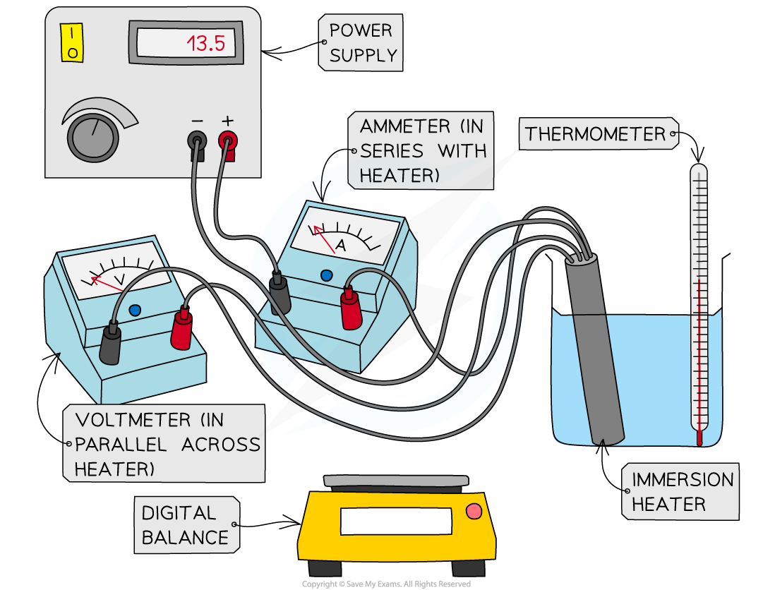
Apparatus for heating water and measuring energy supplied
Key points
- The kit comprises a balance, insulated beaker, immersion heater, voltmeter, ammeter, stopwatch and thermometer.
- The mass of water is measured on the balance before heating begins.
- The heater is switched on and the meters read at the same time as the stopwatch starts.
- Temperature readings are taken at regular intervals while the heater runs.
- The set-up keeps the heater fully submerged so all delivered energy enters the water.
First pass
Weigh the water, drop in the heater, wire up the meters, and switch on while starting the clock. Note the temperature every half-minute and read the meters so the energy can be counted.
Analogy — A cooking show with a scoreboard: the balance weighs the pot, the meters count the gas, the thermometer reports the result every round.
Exam pointer — Method marks live in the sequence: mass first, then meters zeroed and read, then heating with timed temperature readings — describe the order, not just the list.
Going deeper
The apparatus couples electrical metering to thermal sensing so that ΔQ is known independently of the water's properties. Full submersion and lagging minimise the two leakage classes — energy bypassing the water and heat escaping to air — while fixed-interval sampling turns the run into an energy-versus-temperature dataset suitable for a gradient method.
Analogy — An audit trail: every joule is receipted by the meters (VIt), every degree is receipted by the thermometer, and the auditor (the calculation) compares the two books.
Exam pointer — Quote the insulation purpose explicitly — lagging reduces the systematic error of heat lost to the surroundings, which otherwise inflates the measured capacity.
Checks
0 of 9 attempted · 0 correct
3.Results table and the energy ledger
The results live in two books: the meters' energy ledger and the thermometer's temperature column. Tabulating both against time lets every joule be matched to every degree at the moment it arrived.
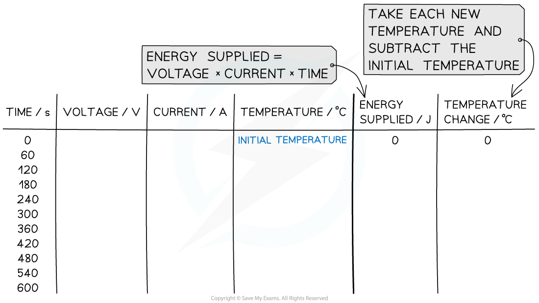
An example of a suitable results table for the specific heat capacity experiment looks like this. Energy supplies = voltage x current x time.
Key points
- The table records time, temperature, and the meter readings at each interval.
- Energy supplied is accumulated as voltage × current × elapsed time.
- Each temperature is paired with the energy delivered up to that moment.
- The energy-per-degree relationship becomes visible once the table is complete.
First pass
Every half-minute, write down the clock, the temperature, and the meters. Multiply voltage by current by the seconds elapsed to stack up the energy next to each temperature.
Analogy — A shared spreadsheet: one column counts money in (energy), another counts the rise it bought (temperature), and each row is a receipt.
Exam pointer — The table earns marks when the energy column is cumulative and aligned with each temperature — a mismatched ledger loses the analysis marks later.
Going deeper
Structuring the table with a cumulative energy column converts the run into paired (ΔQ, ΔT) points suitable for plotting energy against temperature rise. Because ΔQ = mcΔT, the gradient of that plot equals m × c, so the ledger format feeds directly into the gradient analysis rather than relying on a single end-point ratio.
Analogy — Mileage versus fuel burned, logged at every petrol stop: the slope of the log reveals the car's consumption far better than one end-to-end division.
Exam pointer — If the table shows the temperature levelling while energy keeps flowing, suspect a state change or a heater fault — do not force the linear analysis through curved data.
Checks
0 of 9 attempted · 0 correct
4.Analysis by gradient, evaluation and safety
Plot the ledger and the slope speaks: gradient one over mass times capacity gives the answer, provided the joules all landed — which is where losses, repetition and mains safety take over the evaluation.
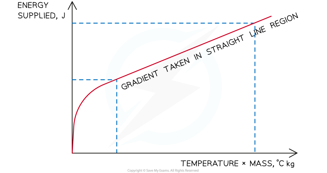
The gradient of the graph is equal to the specific heat capacity of the substance, assuming a perfectly efficient immersion heater
Key points
- Plot temperature rise on the vertical axis against energy supplied on the horizontal axis.
- The gradient of the line equals 1 ÷ (m × c), so c = 1 ÷ (m × gradient).
- Heat lost to the surroundings is the main systematic error and makes the measured c too high.
- Lagging the beaker and fully submerging the heater cut the dominant systematic loss.
- Parallax and reaction-time wobble are random errors, reduced by repetition and smoothing.
- Mains heaters demand dry hands, insulated leads, eye protection and safe handling of scalding water.
First pass
Take the slope, divide one by mass times slope, and the capacity appears — as long as no joules leaked, so lag the beaker, repeat the run, and keep the mains wiring dry and guarded.
Analogy — A scales-and-tilt audit: read the honest line (gradient), fence off the leak (lagging), take several weighings (repetition), and keep the plug socket dry throughout.
Exam pointer — Order the evaluation: name the error, give its direction on c, then the fix — and keep every mains-safety point separate from the thermal analysis.
Going deeper
Rearranging ΔQ = mcΔT gives ΔT = (1/mc)·ΔQ, so the fitted slope yields c for the fixed mass; the dominant systematic term is unaccounted power dissipated outside the sample, biasing c upward, while parallax and timing scatter are random and average out over repeats. Mains safety — dry hands, insulated leads, supervised switching — is a separate, non-negotiable layer.
Analogy — Auditing a delivery route: the odometer counts every kilometre including detours, so the true fuel-per-kilometre needs the detours fenced (lagging) and several runs averaged (repetition) — all with the driver gloved and grounded.
Exam pointer — Distinguish the two bias directions before naming fixes: losses and an underestimated rise both inflate c, while a mass overestimate would deflate it — then separate the mains-safety list from the thermal list.
Checks
0 of 9 attempted · 0 correct
Guided content from the SME authoring corpus — note rn_KQ2Z3k364fVw9Gkq, pinned at 8788fc85a2c1 · promoted SyllabAI/syllabai-resources b3caaaa90c5e