Can we sketch these four related curves?

Can we sketch these four related curves?

Question

Sketch, on separate diagrams, the curves $\text{(i)}\ y=\frac{x-a}{x},\qquad \text{(ii)}\ y=\frac{x^2-a^2}{x^2},$ where $a$ is a positive constant.

[The equations of any asymptotes should be stated, together with the coordinates of any intersections with the axes.]

Hence sketch the curves $\text{(iii)}\ y = \left|\frac{x-a}{x}\right|,\qquad \text{(iv)}\ y^2 = \frac{x^2-a^2}{x^2}.$

Suggestion

When sketching curves, it is helpful to ask:

1. Where are the intersections with the axes?
2. What happens as $x$ tends to $\pm \infty$? Are there horizontal asymptotes? Asymptotes at an angle?
3. What are the vertical asymptotes?
4. Are there any stationary points?
5. Is there any symmetry?

Can we write our equation for (i) as $y=p+\frac{q}{x}$ for some $p$ and $q$?

Can we view this as the combination of two transformations of a simpler curve?

How is our equation for (ii) similar to that for (i)? How is it different?

Will these functions look similar to the ones from the first part at all?

Solution (i)+(ii)

Sketch, on separate diagrams, the curves $\text{(i)}\ y=\frac{x-a}{x},\qquad \dots$ where $a$ is a positive constant.

[The equations of any asymptotes should be stated, together with the coordinates of any intersections with the axes.]

We begin by rewriting the given function as

$$\begin{equation} y=1-\frac{a}{x}. \end{equation}$$

When sketching curves, a useful strategy in many cases is to see if the function can be written in terms of other functions whose graphs we already know.

In this case, we can start by considering the graph of the basic function $\frac{1}{x}$. It has a vertical asymptote at $x=0$ and a horizontal asymptote at $y=0$.

We will now try to manipulate this curve until we obtain the graph of equation $(1)$. Multiplying the curve by $-1$ is a reflection in the $x$-axis. This gives us the curve $y=-\frac{1}{x}$, as shown below. We note that the equations of the asymptotes are the same in this case.

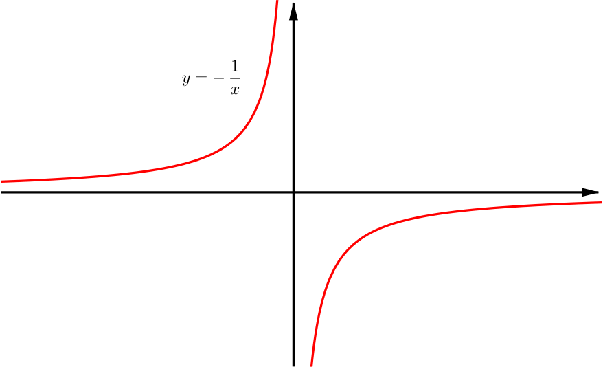
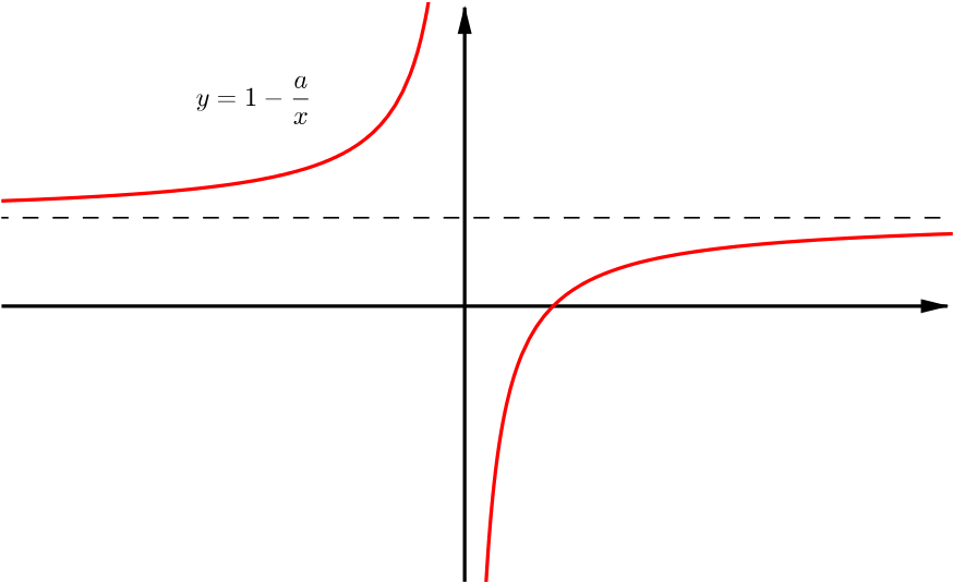
Next we consider multiplication by $a$. As $a$ is a positive constant, this can be interpreted as a stretching in the $y$-direction by a factor of $a$ and so only has the effect of changing the scale on the graph.

We now note that addition by a constant is equivalent to a shift of its graph in the $y$-direction. In the sketch below we see the graph of $y=1-\frac{a}{x}$, as required. The asymptotes are also translated by $1$ in the $y$-direction and so the equations of the new asymptotes are $y=1$ and $x=0$. We also note that the curve intersects the $x$-axis when $x=a$, by substituting $y=0$ into the equation.

Sketch, on separate diagrams, the curves $\dots,\qquad \text{(ii)}\ y=\frac{x^2-a^2}{x^2},$ where $a$ is a positive constant.

[The equations of any asymptotes should be stated, together with the coordinates of any intersections with the axes.]

As with (i), we begin by rewriting the equation as

$$\begin{equation} y=1-\frac{a^2}{x^2}. \end{equation}$$

Similarly to before, we aim to sketch the graph of $y=\frac{1}{x^2}$ and then use tranformations until we obtain the graph of equation $(2)$.

We know that the graph of $y=\frac{1}{x^2}$ must be similar to that of $y=\frac{1}{x}$, with smaller values increasing their distance from the $x$-axis and larger values decreasing their distance from the $x$ axis. The $y$ values are also positive and so any negative parts of the graph are reflected upwards in the $x$-axis.

Multiplication by $-a^2$ is a reflection in the $x$-axis followed by a stretch by a factor of $a^2$ in the $y$ direction.

Finally, addition by $1$ shifts the graph upwards by one unit. We also note that the curve intersects the $x$-axis at the points $x=a$ and $x=-a$, by substituting $y=0$ into equation $(2)$. Similarly to before, our final asymptotes are also shifted upwards by one unit and so are $y=1$ and $x=0$.

Is there a way to use the graph of $y=\frac{x-a}{x}$ to sketch this curve directly?

Solution (iii)+(iv)

Hence sketch the curves $\text{(iii)}\ y = \left|\frac{x-a}{x}\right|,\qquad \dots$

As we already have a sketch of the graph $y=\frac{x-a}{x}$, we need only consider the effect that taking the absolute value has on the graph.

Every point on the curve with a positive $y$ co-ordinate is fixed and every point with a negative $y$ co-ordinate is reflected in the $x$-axis. This gives us the following sketch.

Hence sketch the curves $\dots,\qquad \text{(iv)}\ y^2 = \frac{x^2-a^2}{x^2}.$

Approach 1

We start by rewriting our equation as

$$\begin{equation} y=\pm \sqrt{1-\frac{a^2}{x^2}}. \end{equation}$$

Firstly, we note that if $-a<x<a$, then $1-\frac{a^2}{x^2} <0$ and so ((equation)) has no solutions. This means that our curve only has points with $x\ge a$ or $x \le -a$. We will consider the sketch of $y=1-\frac{a^2}{x^2}$, from (ii), in this range and aim to plot the square roots. This is, for each point $(x,y)$ on this curve, we want to include the points $(x,\pm \sqrt{y})$ in our sketch of ((equation)).

If $y<1$, then the vertical distance decreases and, if $y>1$, the vertical distance increases. Therefore, we get the following graph for the positive root $y=+\sqrt{1-\frac{a^2}{x^2}}$.

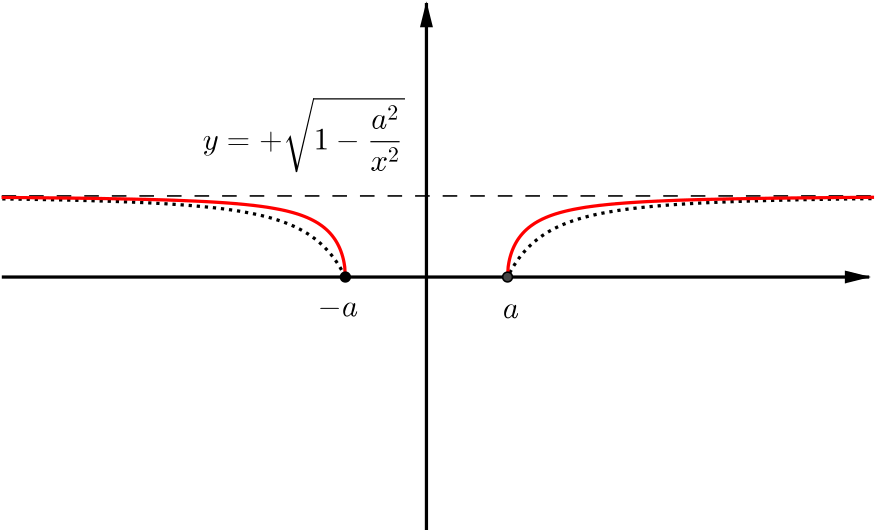
To plot the other root $y=-\sqrt{1-\frac{a^2}{x^2}}$, we can simply add the reflection in the $x$-axis.

We now need only consider the points $(\pm a,0)$ and the angles that the curves make at these points. Comparing to the graph of $y=\sqrt{x}$, we would not expect the curve to be sharp at these points. Hence, we will include the information that the curve intersects the $x$-axis at right-angles in our final sketch.

Similarly to before, the equations of the asymptotes are $y=\pm 1$ and the points of intersection are at $x=\pm a$.

The full details as to why this argument works will be touched on at university-level, but there are a number of ways that we can convince ourselves of this result none-the-less. For example, would we expect these points to be sharp if we rewrote the curve in the form $x=\pm\frac{a}{\sqrt{1-y^2}}$? Alternatively, what would we expect if we used calculus to calculate the gradient of the curve at these points? What does this tell us?

Approach 2

We begin by rewriting our equation as

$$\begin{equation} y^2 + \left(\frac{a}{x}\right)^2 = 1. \end{equation}$$

As this looks similar to the equation for a circle, we will begin by considering the graph of the unit circle $y^2+x^2=1$.

To get the graph of equation $(4)$, we want to swap the $x$ for $\frac{a}{x}$. This is equivalent to finding another point $x'$ such that $xx'=a$ (i.e. point $x'$ for which the geometric mean of $x$ and $x'$ are on the lines $x=\pm\sqrt{a}$). This is equivalent to inversion in the lines $x=\pm\sqrt{a}$ and so each half of the circle can be projected outwards in the $x$-direction, as shown.